Diff-in-Diff as an identification strategy

Parallel trend assumption (PTA)

Estimate Average Treatment Effect on the Treated (ATT)

But what if the PTA doesn't hold?

But what if the PTA doesn't hold?

We can potentially remove [part of] the bias by matching on X^s_it=X_i

This paper

• Identify contexts when matching can recover causal estimates under certain violations of the parallel trend assumption.

  • Overall bias reduction and increase in robustness for sensitivity analysis.

• Use mixed-integer programming matching (MIP) to balance covariates directly.
  
  

DD Setup

• Let $Y_{it}\left(z\right)$ be the potential outcome for unit $i$ in period $t$ under treatment $z$.

• Intervention implemented in $T_0$ $\to$ No units are treated in $t\le T_0$

• Difference-in-Differences (DD) focuses on ATT for $t>T_0$:

$$ATT\left(t\right)=E\left[Y_{it}\right(1)-Y_{it}(0)|Z=1]$$

DD Setup

• Let $Y_{it}\left(z\right)$ be the potential outcome for unit $i$ in period $t$ under treatment $z$.

• Intervention implemented in $T_0$ $\to$ No units are treated in $t\le T_0$

• Difference-in-Differences (DD) focuses on ATT for $t>T_0$:

$$ATT\left(t\right)=E\left[Y_{it}\right(1)-Y_{it}(0)|Z=1]$$

• Under the PTA:

$$\begin{array}{cc}{\hat{\tau }}^{DD}=& \stackrel{{\Delta }_{post}}{\stackrel{}{E[Y_{i1}|Z=1]-E[Y_{i1}|Z=0]}}-\\ & \underset{{\Delta }_{pre}}{\underset{}{\left(E\right[Y_{i0}|Z=1]-E[Y_{i0}|Z=0\left]\right)}}\end{array}$$

Bias in a DD setting

Bias can be introduced to DD in different ways:

1) Time-invariant covariates with time-varying effects: Obs. Bias

• e.g. Effect of gender on salaries.

2) Differential time-varying effects: Obs. Diff. Bias

• e.g. Effect of race on salaries evolve differently over time by group.

3) Observed or unobserved time-varying covariates: Unobs. Bias

• e.g. Test scores

If the PTA holds...

$$\begin{array}{cc}\stackrel{Obs.Bias}{\stackrel{}{\left({\overline{\gamma }}_1\right(X^1,t^{\prime })-{\overline{\gamma }}_1(X^0,t^{\prime }\left)\right)-\left({\overline{\gamma }}_1\right(X^1,t)-{\overline{\gamma }}_1(X^0,t\left)\right)}}+& \\ \underset{Obs.Diff.Bias}{\underset{}{\left({\overline{\gamma }}_2\right(X^1,t^{\prime })-{\overline{\gamma }}_2(X^1,t\left)\right)}}+\underset{Unobs.Bias}{\underset{}{({\lambda }_{t^{\prime }1}-{\lambda }_{t^{\prime }0})-({\lambda }_{t1}-{\lambda }_{t0})}}& =0\end{array}$$

Sensitivity analysis for Diff-in-Diff

• In an event study $\to$ null effects prior to the intervention:

Honest approach to test pretrends

• One main issue with the previous test $\to$ Underpowered

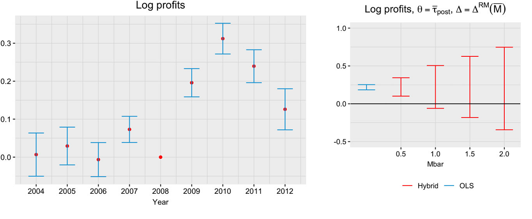
• Rambachan & Roth (2023) propose sensitivity bounds to allow pre-trends violations:

  • E.g. Violations in the post-intervention period can be at most $M$ times the max violation in the pre-intervention period.

Different scenarios

For linear and quadratic functions:

S1: No interaction between X and t

S2: Equal interaction between X and t

S3: Differential interaction between X and t

S4: S3 + Bias cancellation

• For all scenarios, differential distribution of covariates $X$ between groups

Parameters:

• Estimate compared to sample ATT (can be different for matching)

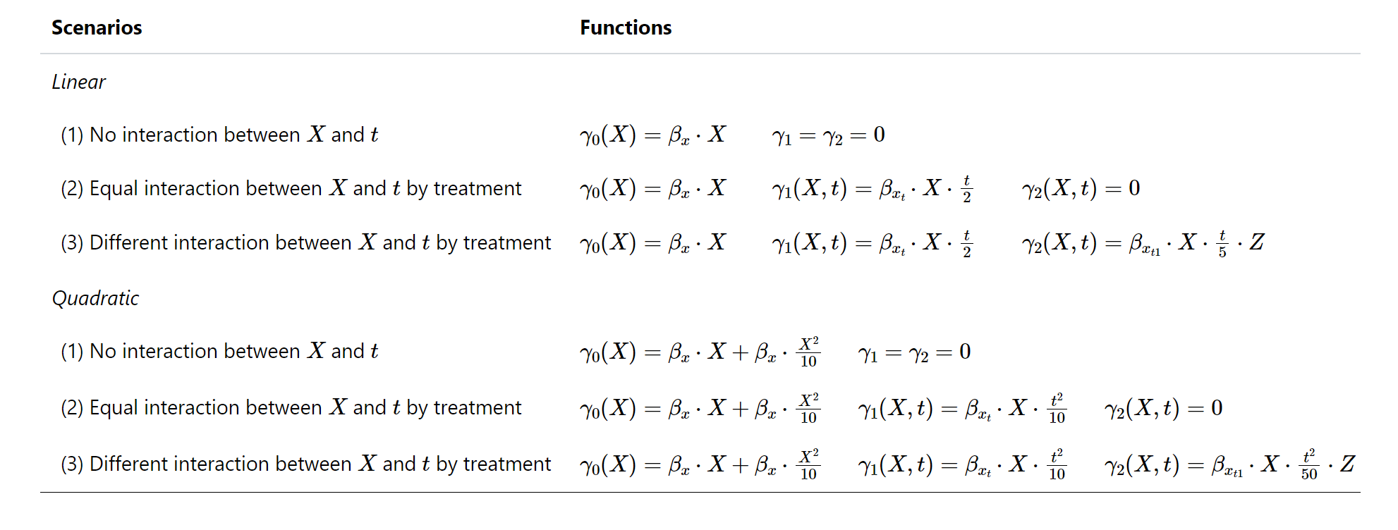
S1 - No interaction between X and t

S2 - Equal interaction between X and t by treatment

S3 - Differential interaction between X and t by treatment

Why is this bias reduction important?

• Example of S2 (Quadratic) with no true effect:

Why is this bias reduction important?

• Even under modest bias, we would incorrectly reject the null 20% of the time.

Why is this bias reduction important?

• Sensitivity analysis results are skewed by the magnitude of the bias.

S4: Bias cancellation

Preferential Voucher Scheme in Chile

• Universal flat voucher scheme $\stackrel{2008}{⟶}$ Universal + preferential voucher scheme

• Preferential voucher scheme:

  • Targeted to bottom 40% of vulnerable students

  • Additional 50% of voucher per student

  • Additional money for concentration of SEP students.

Before matching: Household income

Before matching: Average SIMCE

Matching + DD

• Prior to matching: No parallel pre-trend

• Different types of schools:

  • Schools that charge high co-payment fees.

  • Schools with low number of SEP student enrolled.

• MIP Matching using constant or "sticky" covariates:

  • Mean balance (0.025 SD): Enrollment, average yearly subsidy, number of voucher schools in county, charges add-on fees

  • Exact balance: Geographic province

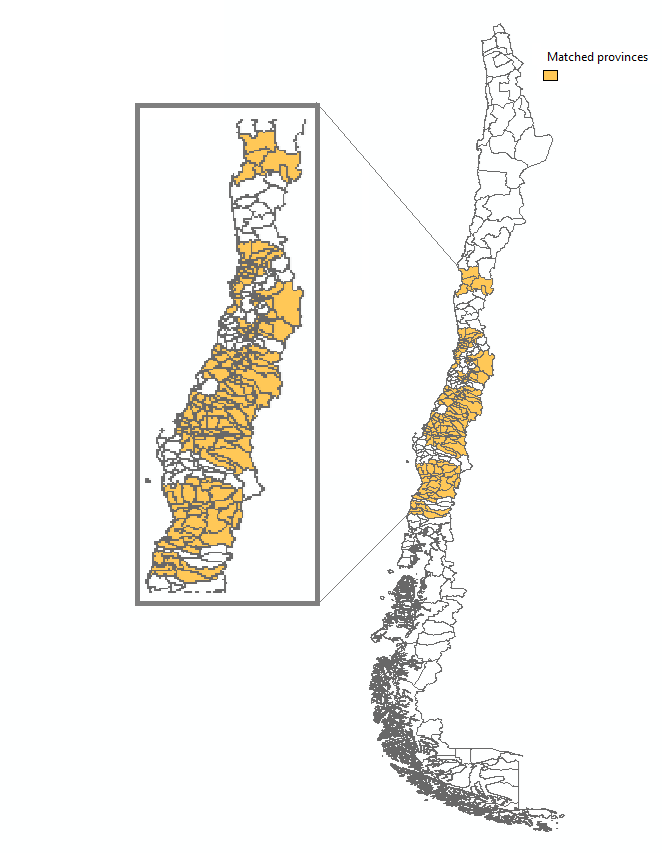
Groups are balanced in specific characteristics

Matching in 16 out of 53 provinces

After matching: Household income

After matching: Average SIMCE

Results

• Matched schools:

  • More vulnerable and lower test scores than the population mean.

• 9pp increase in the income gap between SEP and non-SEP schools in matched DD:

  • SEP schools attracted even more vulnerable students.

  • Non-SEP schools increased their average family income.

• No evidence of increase in SIMCE score:

  • Could be a longer-term outcome.

• Findings in segregation are moderately robust to hidden bias (Keele et al., 2019):

  • ${\Gamma }_c=1.76$ $\to$ Unobserved confounder would have to change the probability of assignment from 50% vs 50% to 32.7% vs 67.3%.

  • Allows up to 70% of the maximum deviation in the pre-intervention period (M = 0.7) vs 50% without matching (Rambachan & Roth, 2023)

Potential reasons?

• Increase in probability of becoming SEP in 2009 jumps discontinuously at 60% of SEP student concentration in 2008 (4.7 pp; SE = 0.024)

Conclusions and Next Steps

Honest approach to test pretrends

• One drawback of the previous method is that it can overstate (or understate) the robustness of findings if the point estimate is biased.

  • Honest CIs depend on the magnitude of the point estimate as well as the pre-trend violations.
    

• Matching can reduce the overall bias of the point estimate

  

How do we match?

• Match on covariates or outcomes? Levels or trends?

• Propensity score matching? Optimal matching? etc.

This paper:

• Match on time-invariant covariates that could make groups behave differently.

  • Use distribution of covariates to match on a template.

• Use of Mixed-Integer Programming (MIP) Matching (Zubizarreta, 2015; Bennett, Zubizarreta, & Vielma, 2020):

  • Balance covariates directly

  • Yield largest matched sample under balancing constraints (cardinality matching)

  • Works fast with large samples

Data Generating Processes

SEP adoption over time