class: inverse, center, middle <br> <br> <br> <h1 class="title-own">Difference-in-Differences<br/>using Mixed-Integer Programming Matching Approach</h1> <br> <br> .small[Magdalena Bennett <br>*McCombs School of Business, The University of Texas at Austin* ] <br> .small[Seminario DIIS - PUC<br>November 20th, 2024] --- # Diff-in-Diff as an identification strategy <img src="mbennett_ddmatch_files/figure-html/dd-1.svg" style="display: block; margin: auto;" /> --- # Cannot compare treated vs control <img src="mbennett_ddmatch_files/figure-html/dd_tc-1.svg" style="display: block; margin: auto;" /> --- # Cannot compare before and after <img src="mbennett_ddmatch_files/figure-html/dd_ba-1.svg" style="display: block; margin: auto;" /> --- # Parallel trend assumption (PTA) <img src="mbennett_ddmatch_files/figure-html/dd2-1.svg" style="display: block; margin: auto;" /> --- # Estimate Average Treatment Effect on the Treated (ATT) <img src="mbennett_ddmatch_files/figure-html/dd3-1.svg" style="display: block; margin: auto;" /> --- # Diff-in-Diff is very popular in Economics <img src="mbennett_ddmatch_files/figure-html/gg-1.svg" style="display: block; margin: auto;" /> .source[Source: Web of Science (11/18/2024)] --- # Diff-in-Diff is very popular in Economics <img src="mbennett_ddmatch_files/figure-html/gg2-1.svg" style="display: block; margin: auto;" /> .source[Source: Web of Science (11/18/2024)] --- # What about parallel trends? .pull-left[ .center[ ] ] .pull-right[] --- # What about parallel trends? .pull-left[ .center[ ] ] .pull-right[ - Main identification assumption **.darkorange[fails]**] --- # What about parallel trends? .pull-left[ .center[ ] ] .pull-right[ - Main identification assumption **.darkorange[fails]** - Find sub-groups that potentially **.darkorange[follow PTA]** - E.g. similar units in treatment and control - Similar to synthetic control intuition. ] --- # What about parallel trends? .pull-left[ .center[ ] ] .pull-right[ - Main identification assumption **.darkorange[fails]** - Find sub-groups that potentially **.darkorange[follow PTA]** - E.g. similar units in treatment and control - Similar to synthetic control intuition. - Can matching help? - It's **.darkorange[complicated]** .small[(Ham & Miratrix, 2022; Zeldow & Hatfield, 2021; Basu & Small, 2020; Lindner & McConnell, 2018; Daw & Hatfield, 2018 (x2); Ryan, 2018; Ryan et al., 2018)] ] --- # This paper - Identify contexts when matching can recover causal estimates under **.darkorange[certain violations of the parallel trend assumption]**. - Overall bias reduction and increase in robustness for sensitivity analysis. - Use **.darkorange[mixed-integer programming matching (MIP)]** to balance covariates directly. -- <br/> <br/> .pull-left[ .box-6trans[**Simulations:**<br/>Different DGP scenarios] ] .pull-right[ .box-6trans[**Application:**<br/>School segregation & vouchers] ] --- background-position: 50% 50% class: left, bottom, inverse .big[ Let's get started <br> <br> ] --- # DD Setup - Let `\(Y_{it}(z)\)` be the potential outcome for unit `\(i\)` in period `\(t\)` under treatment `\(z\)`. - Intervention implemented in `\(T_0\)` `\(\rightarrow\)` No units are treated in `\(t\leq T_0\)` -- - Difference-in-Differences (DD) focuses on ATT for `\(t>T_0\)`: `$$ATT(t) = E[Y_{it}(1) - Y_{it}(0)|Z=1]$$` -- .box-6trans[Expected difference in potential outcomes<br>*if the treatment hadn't happened*<br>**for the treatment group**] --- # DD Setup - Let `\(Y_{it}(z)\)` be the potential outcome for unit `\(i\)` in period `\(t\)` under treatment `\(z\)`. - Intervention implemented in `\(T_0\)` `\(\rightarrow\)` No units are treated in `\(t\leq T_0\)` - Difference-in-Differences (DD) focuses on ATT for `\(t>T_0\)`: `$$ATT(t) = E[Y_{it}(1) - Y_{it}(0)|Z=1]$$` - **.darkorange[Assumptions for DD]**: - Parallel-trend assumption (PTA) - Common shocks `$$E[Y_{i1}(0) - Y_{i0}(0) | Z=1] = E[Y_{i1}(0) - Y_{i0}(0) | Z=0]$$` --- # DD Setup (cont.) - Under these assumptions: $$ `\begin{align} \hat{\tau}^{DD} = &\color{#FFC857}{\overbrace{\color{black}{E[Y_{i1}|Z=1] - E[Y_{i1}|Z=0]}}^{\color{#FFC857}{\Delta_{post}}}} - \\ &\color{#CBB3BF}{\underbrace{\color{black}{(E[Y_{i0}|Z=1] - E[Y_{i0}|Z=0])}}_{\color{#CBB3BF}{\Delta_{pre}}}} \end{align}` $$ - Where `\(t=0\)` and `\(t=1\)` are the pre- and post-intervention periods, respectively. - `\(Y_{it} = Y_{it}(1)\cdot Z_i + (1-Z_i)\cdot Y_{it}(0)\)` is the observed outcome. --- # But what if the PTA doesn't hold? <br> <br> .pull-left[ <img src="mbennett_ddmatch_files/figure-html/po1-1.svg" style="display: block; margin: auto;" /> ] --- # But what if the PTA doesn't hold? .box-6trans[We can potentially remove [part of] the bias by matching on <i>X<sup>s</sup><sub>it</sub>=X<sub>i</sub></i>] .pull-left[ <img src="mbennett_ddmatch_files/figure-html/po2-1.svg" style="display: block; margin: auto;" /> ] .pull-right[ <img src="mbennett_ddmatch_files/figure-html/po3-1.svg" style="display: block; margin: auto;" /> ] --- # General form of potential outcomes We can write a general form of the potential outcomes `\(Y(0)\)` and `\(Y(1)\)` as follows: `$$Y_{it}(0) = \alpha_i + \lambda_{t} + \gamma_0(X_{i}) + \gamma_1(X_i,t) + \gamma_2(X_i,t)\cdot Z_i + u_{it}$$` `$$Y_{it}(1) = Y_{it}(0) + \tau_{it} = \alpha_i + \lambda_t + \gamma_0(X_{i}) + \gamma_1(X_i,t) + \gamma_2(X_i,t)\cdot Z_i + \tau_{it} + u_{it}$$` -- .box-6trans[Covariate distribution between groups can be **different**<br>$$X_i|Z \sim F_x(z)$$] --- # General form of potential outcomes We can write a general form of the potential outcomes `\(Y(0)\)` and `\(Y(1)\)` as follows: `$$Y_{it}(0) = \color{#119DA4}{\mathbf{\alpha_i + \lambda_{t}}} + \gamma_0(X_{i}) + \gamma_1(X_i,t) + \gamma_2(X_i,t)\cdot Z_i + u_{it}$$` - `\(\alpha_i\)` and `\(\lambda_t\)` are individual and time FE, respectively. - If `\(\lambda_t|Z \sim F_{\lambda}(z,t)\)`, then PTA fails. --- # General form of potential outcomes We can write a general form of the potential outcomes `\(Y(0)\)` and `\(Y(1)\)` as follows: `$$Y_{it}(0) = \alpha_i + \lambda_{t} + \color{#119DA4}{\mathbf{\gamma_0(X_{i})}} + \gamma_1(X_i,t) + \gamma_2(X_i,t)\cdot Z_i + u_{it}$$` .darkgrey[- `\(\alpha_i\)` and `\(\lambda_t\)` are individual and time FE, respectively. - If `\(\lambda_t|Z \sim F_{\lambda}(z,t)\)`, then PTA fails.] - `\(\gamma_0(X_i)\)` is a time-invariant function that associates `\(X\)` and `\(Y\)` --- # General form of potential outcomes We can write a general form of the potential outcomes `\(Y(0)\)` and `\(Y(1)\)` as follows: `$$Y_{it}(0) = \alpha_i + \lambda_{t} + \gamma_0(X_{i}) + \color{#119DA4}{\mathbf{\gamma_1(X_i,t)}} + \gamma_2(X_i,t)\cdot Z_i + u_{it}$$` .darkgrey[- `\(\alpha_i\)` and `\(\lambda_t\)` are individual and time FE, respectively. - If `\(\lambda_t|Z \sim F_{\lambda}(z,t)\)`, then PTA fails. - `\(\gamma_0(X_i)\)` is a time-invariant function that associates `\(X\)` and `\(Y\)`.] - `\(\gamma_1(X_i,t)\)` is a time-dependent function. --- # General form of potential outcomes We can write a general form of the potential outcomes `\(Y(0)\)` and `\(Y(1)\)` as follows: `$$Y_{it}(0) = \alpha_i + \lambda_{t} + \gamma_0(X_{i}) + \gamma_1(X_i,t) + \color{#119DA4}{\mathbf{\gamma_2(X_i,t)\cdot Z_i}} + u_{it}$$` .darkgrey[- `\(\alpha_i\)` and `\(\lambda_t\)` are individual and time FE, respectively. - If `\(\lambda_t|Z \sim F_{\lambda}(z,t)\)`, then PTA fails. - `\(\gamma_0(X_i)\)` is a time-invariant function that associates `\(X\)` and `\(Y\)`. - `\(\gamma_1(X_i,t)\)` is a time-dependent function.] - `\(\gamma_2(X_i,t)\cdot Z_i\)` is a _differential_ time-dependent function **only** for the treatment group. --- # If the PTA holds... Then, for a 2x2 DD, where `\(t<T_0\)` (pre) and `\(t'>T_0\)` (post): `$$\mathbb{E}[\gamma_1(X_{i}, t') + \gamma_2(X_{i}, t') - \gamma_1(X_{i}, t) - \gamma_2(X_{i}, t)|Z=1] = \mathbb{E}[\gamma_1(X_{i}, t') - \gamma_1(X_{i}, t)|Z=0]$$` -- **.darkorange[One of the two]** conditions need to hold: 1) No effect or constant effect of `\(X\)` on `\(Y\)` over time: `\(\mathbb{E}[\gamma_1(X,t)] = \mathbb{E}[\gamma_1(X)]\)` 2) Equal distribution of observed covariates between groups: `\(X_i|Z=1 \overset{d}{=} X_i|Z=0\)` -- <br> **.darkorange[in addition to]**: 3) No differential time effect of `\(X\)` on `\(Y\)` by treatment group: `\(\mathbb{E}[\gamma_2(X,t)] = 0\)` -- <br> .pull-left[ .box-6trans[**Cond. 2** can hold through **matching**] ] -- .pull-right[ .box-6trans[**Cond. 3** can be tested with **sensitivity analysis**] ] --- # Sensitivity analysis for Diff-in-Diff - Use of **.darkorange[pre-trends]** to test plausibility of the PTA: <img src="mbennett_ddmatch_files/figure-html/dd_placebo-1.svg" style="display: block; margin: auto;" /> --- # Sensitivity analysis for Diff-in-Diff - Using a diff-in-diff strategy, we shouldn't find an effect <img src="mbennett_ddmatch_files/figure-html/dd_placebo2-1.svg" style="display: block; margin: auto;" /> --- # Sensitivity analysis for Diff-in-Diff - In an event study `\(\rightarrow\)` null effects prior to the intervention: <img src="mbennett_ddmatch_files/figure-html/dd_placebo3-1.svg" style="display: block; margin: auto;" /> --- # Honest approach to test pretrends - One main issue with the previous test `\(\rightarrow\)` **.darkorange[Underpowered]** -- - Rambachan & Roth (2023) propose **.darkorange[sensitivity bounds]** to allow pre-trends violations: - E.g. Violations in the post-intervention period can be _at most_ `\(M\)` times the max violation in the pre-intervention period. -- .center[ 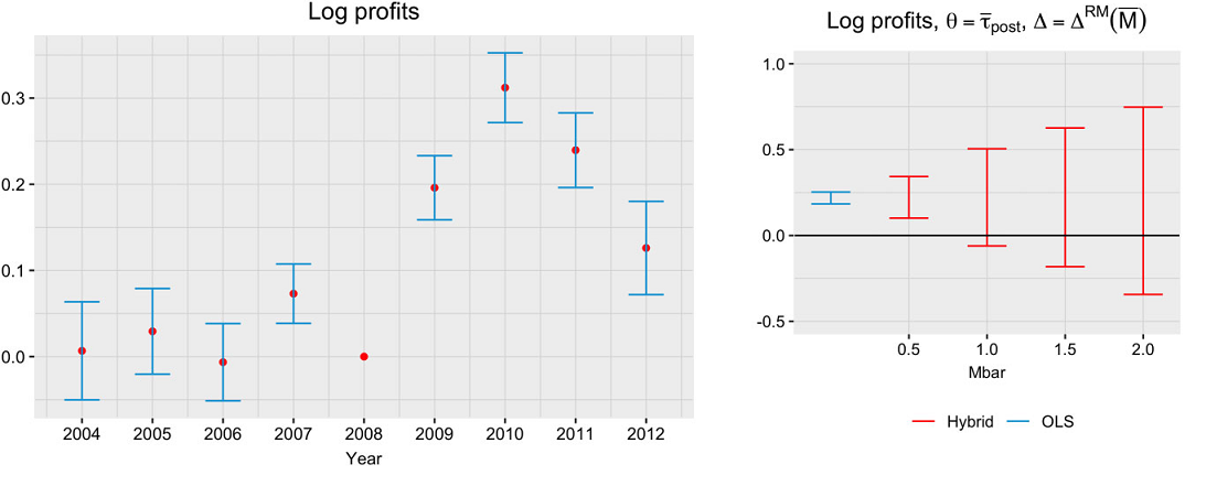] --- # Honest approach to test pretrends - One drawback of the previous method is that it can **.darkorange[overstate]** (or understate) the robustness of findings if the point estimate is biased. - Honest CIs depend on the **.darkorange[magnitude of the point estimate]** as well as the **.darkorange[pre-trend violations]**. -- <br> - Matching can **.darkorange[reduce the overall bias]** of the point estimate -- .center[  ] --- # How do we match? - Match on covariates or outcomes? Levels or trends? - Propensity score matching? Optimal matching? etc. -- This paper: - **.darkorange[Match on time-invariant covariates]** that could make groups behave differently. - Use distribution of covariates to match on a template. - Use of **.darkorange[Mixed-Integer Programming (MIP) Matching]** .small[(Zubizarreta, 2015; Bennett, Zubizarreta, & Vielma, 2020)]: - Balance covariates directly - Yield largest matched sample under balancing constraints (cardinality matching) - Works fast with large samples --- background-position: 50% 50% class: left, bottom, inverse .big[ Simulations <br> <br> ] --- # Different scenarios For linear and quadratic functions: <br> .box-1trans[S1: No interaction between X and t] .box-2trans[S2: Equal interaction between X and t] .box-3trans[S3: Differential interaction between X and t] Additional tests: <br> .box-4trans[S1b-S3b: Including time-varying covariates] -- <br> - For all scenarios, differential distribution of covariates `\(X\)` between groups --- # Data Generating Processes .center[ 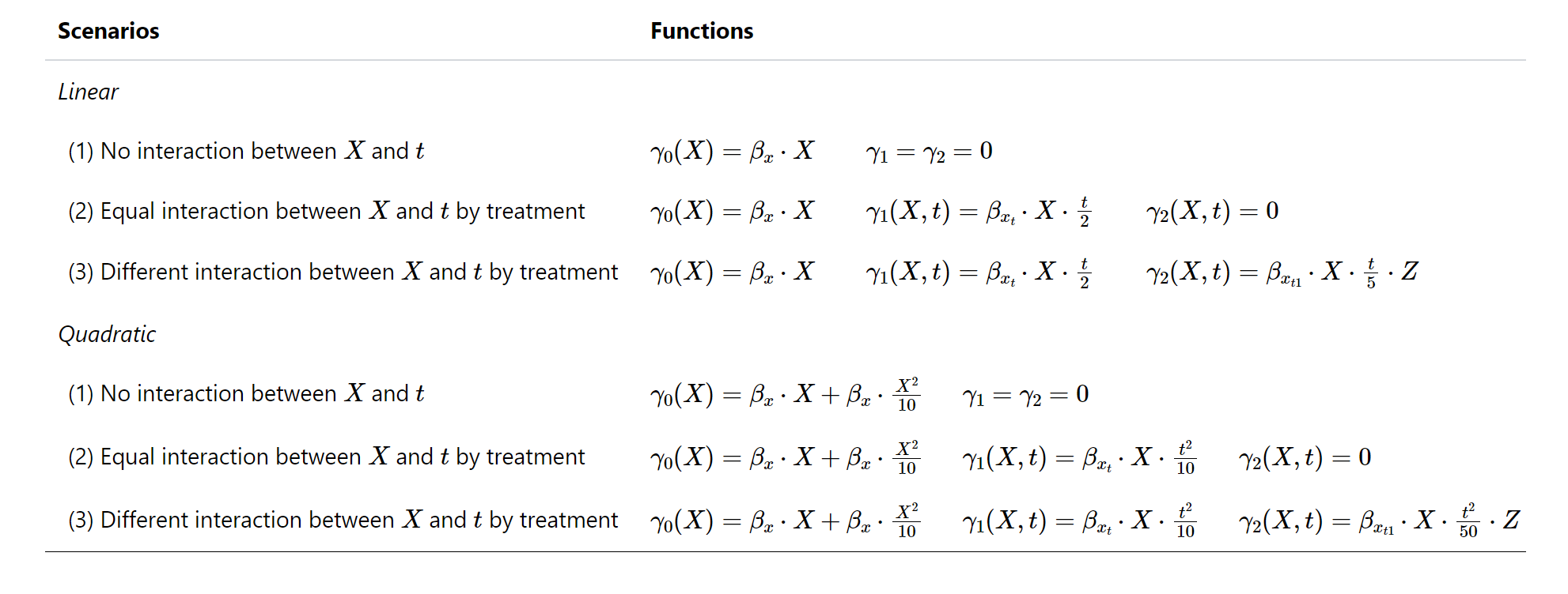 ] --- #Parameters: .center[ Parameter | Value -------------------------------------|---------------------------------------------- Number of obs (N) | 1,000 `Pr(Z=1)` | 0.5 Time periods (T) | 8 Last pre-intervention period (T_0) | 4 Matching PS | Nearest neighbor (using calipers) MIP Matching tolerance | .01 SD Number of simulations | 1,000 ] - Estimate compared to sample ATT (_can be different for matching_) --- # S1 - No interaction between X and t .center[ ] --- # S2 - Equal interaction between X and t by treatment .center[ ] --- # S3 - Differential interaction between X and t by treatment .center[ ] --- # Matching as an adjustment method for reducing/eliminating bias .center[ ] --- # Why is this bias reduction important? - Example of S2 (Quadratic) with no true effect: .center[  ] --- # Why is this bias reduction important? - Even under modest bias, we would incorrectly reject the null 20% of the time. .center[ ] --- # Why is this bias reduction important? - Sensitivity analysis results are skewed by the magnitude of the bias. .center[ ] --- background-position: 50% 50% class: left, bottom, inverse .big[ Application <br> <br> ] --- #Preferential Voucher Scheme in Chile - Universal **.darkorange[flat voucher]** scheme `\(\stackrel{\mathbf{2008}}{\mathbf{\longrightarrow}}\)` Universal + **.darkorange[preferential voucher]** scheme - Preferential voucher scheme: - Targeted to bottom 40% of vulnerable students - Additional 50% of voucher per student - Additional money for concentration of SEP students. -- <br/> .pull-left[ .center[ .box-6trans[**Students:**<br/>- Verify SEP status<br/>- Attend a SEP school] ] ] .pull-right[ .center[ .box-6trans[**Schools:**<br/>- Opt-into the policy<br/>- No selection, no fees<br/>- Resources ~ performance] ] ] --- #Impact of the SEP policy - **.darkorange[Mixed evidence of impact on test scores]** for lower-income students (Aguirre, 2022; Feigenberg et al., 2019; Neilson, 2016; Mizala & Torche, 2013) --- #Impact of the SEP policy - **.darkorange[Mixed evidence of impact on test scores]** for lower-income students (Aguirre, 2022; Feigenberg et al., 2019; Neilson, 2016; Mizala & Torche, 2013) - Design could have **.darkorange[increased]** socioeconomic segregation (E.g. Incentives for concentration of SEP students) --- #Impact of the SEP policy - **.darkorange[Mixed evidence of impact on test scores]** for lower-income students (Aguirre, 2022; Feigenberg et al., 2019; Neilson, 2016; Mizala & Torche, 2013) - Design could have **.darkorange[increased]** socioeconomic segregation (E.g. Incentives for concentration of SEP students) - Key decision variables for schools: Performance, current SEP students, competition, add-on fees. -- - **.darkorange[Diff-in-diff (w.r.t. 2007) for SEP and non-SEP schools]**: - Only for **.darkorange[private-subsidized schools]** - Matching using 2007 variables (similar results when using 2005-2007). - Outcome: Average students' household income and SIMCE score --- #Before matching: Household income .pull-left[  ] .pull-right[  ] --- #Before matching: Average SIMCE .pull-left[  ] .pull-right[  ] --- # Matching + DD - **.darkorange[Prior to matching]**: No parallel pre-trend - **.darkorange[Different types of schools]**: - Schools that charge high co-payment fees. - Schools with low number of SEP student enrolled. - **.darkorange[MIP Matching]** using constant or "sticky" covariates: - Mean balance (0.025 SD): Enrollment, average yearly subsidy, number of voucher schools in county, charges add-on fees - Exact balance: Geographic province --- # Groups are balanced in specific characteristics .center[ ] --- # Matching in 16 out of 53 provinces .center[ 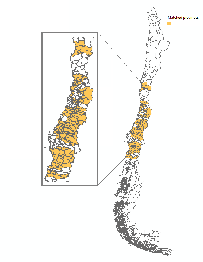] --- # After matching: Household income .pull-left[  ] .pull-right[  ] --- #After matching: Average SIMCE .pull-left[  ] .pull-right[  ] --- #Results - **.darkorange[Matched schools]**: - More vulnerable and lower test scores than the population mean. -- - **.darkorange[9pp increase in the income gap]** between SEP and non-SEP schools in matched DD: - SEP schools attracted even more vulnerable students. - Non-SEP schools increased their average family income. -- - **.darkorange[No evidence of increase in SIMCE score]**: - Could be a longer-term outcome. -- - Findings in segregation are **.darkorange[moderately robust to hidden bias]** (Keele et al., 2019): - `\(\Gamma_c = 1.76\)` `\(\rightarrow\)` Unobserved confounder would have to change the probability of assignment from 50% vs 50% to 32.7% vs 67.3%. - Allows up to 70% of the maximum deviation in the pre-intervention period (*M = 0.7*) vs 50% without matching (Rambachan & Roth, 2023) --- # Potential reasons? - Increase in probability of becoming SEP in 2009 **.darkorange[jumps discontinuously at 60%]** of SEP student concentration in 2008 (4.7 pp; SE = 0.024) .center[ ] --- background-position: 50% 50% class: left, bottom, inverse .big[ Let's wrap it up <br> <br> ] --- # Conclusions and Next Steps .pull-left[ - Matching can be an important tool to address **.darkorange[violations in PTA]**. - **.darkorange[Bias reduction]** is very important for sensitivity analysis. - **.darkorange[Serial correlation]** also plays an important role: Don't match on random noise. - Next steps: Partial identification using time-varying covariates] .pull-right[ .center[ ] ] --- class: inverse, center, middle <br> <br> <br> <h1 class="title-own">Difference-in-Differences<br/>using Mixed-Integer Programming Matching Approach</h1> <br> <br> .small[Magdalena Bennett <br>*McCombs School of Business, The University of Texas at Austin* ] <br> .small[Seminario DIIS - PUC<br>November 20th, 2024] --- # SEP adoption over time .center[  ]